The Grain Size Distribution Estimator Tool is located under the Analysis menu and further the Roughness Analysis sub-menu:

This tool was developed by James Hensleigh as part of the CHaMP program. It is used to produce a surface roughness raster based on CHaMP surveyed channel units with attributes of occular estimates of grain size. It is only appropriate to use for CHaMP surveys and is intended to provide an orthogonal raster input for subsequent hydraulic model analysis or change detection analysis.
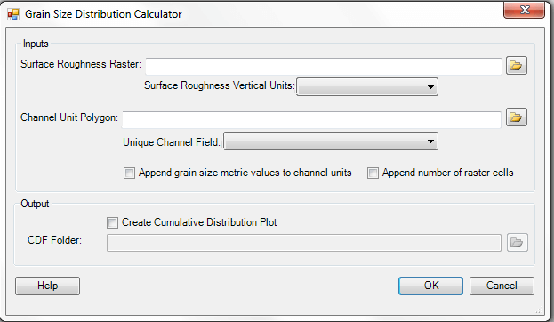
When the Grain Size Distribution Estimator is run, the following dialog appears:

A video tutorial for how to use the Grain Size Distribution Estimator can be seen below:
INPUTS:
The inputs for this tool are:
- Surface roughness raster
- The location and name of the ouput surface roughness raster.
- Vertical units of surface roughness raster
- grain size metrics are generally reported in millimeters so a conversion based on this value is performed to get values in millimeters .
- Channel unit polygon
- Polygon feature class representing areas of interest where the grain size metrics of D16, D50, D84, and D90 will be calculated for.
- Unique channel Field
- Field in polygon feature class that will be used as a unique identifier to append the grain size metrics to the correct field. It is important that the value of this field is a unique for each record in the feature class.
- Append grain size metrics (optional)
- if this check box is selected then the grain size metrics of D16, D50, D84, and D90 will be appended to the channel unit polygon
- Append number of raster cells (optional)
- if this check box is selected then the number of raster cells used to calculate the grain size metrics will be appended to the channel unit polygon.
OUTPUTS:
The outputs for the tool are:
- Create cumulative distribution plot
- if this check box is selected then a cumulative distribution figure of the grain size distribution will be created for each polygon in the channel unit polygon.
- CDF Folder
- The folder to store the cumulative distribution plots to. Each file is named as a combination of the unique field name and its value. For example if a field called Id was used for the unique channel field then the figure for the polygon with an Id of 23 would be named Id_23.png
 Back to TAT Home